Practical Lessons from Predicting Clicks on Ads at Facebook (2014)
In this paper we introduce a model which combines decision trees with logistic regression, outperforming either of these methods on its own by over 3%, an improvement with significant impact to the overall system performance.
We then explore how a number of fundamental parameters impact the final prediction performance of our system.
1. 模型结构
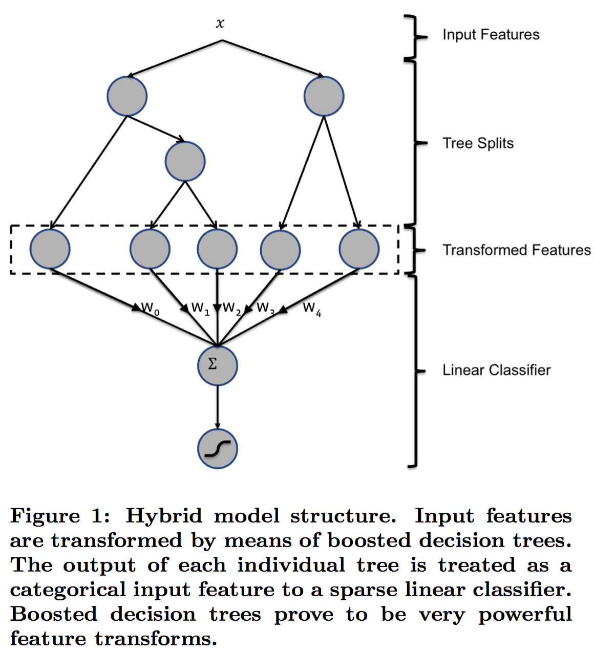
图1 Hybrid model structure
在工业界,LR是CTR的常用模型,而模型的瓶颈主要在于特征工程(特征离散化、特征交叉等),因此模型开发人员需要在特征工程上花费大量的时间与精力。为了解决这个问题,该论文提出的一种模型结构:decision trees + logistic regression,其中decision trees用于feature transformation,而logistic regression用于CTR预测。
该论文在数据集上对decision trees、logistic regression以及decision trees + logistic regression这三种模型进行实验,结果如图2所示。
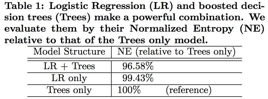
图2 模型对比结果
由图2可知,decision trees + logistic regression模型的结果最优,其主要原因可能有以下几点:
- 与人工特征工程相比,利用decision trees进行feature transformation更有效;
decision trees + logistic regression类似于stacking,在不过拟合的情况下,模型stacking的效果会优于单模型;
2. online learning
论文中提到,data freshness对模型的结果会有影响,如图3所示,delay越小,Normalized Entropy的值越小,即模型预测精度越高。
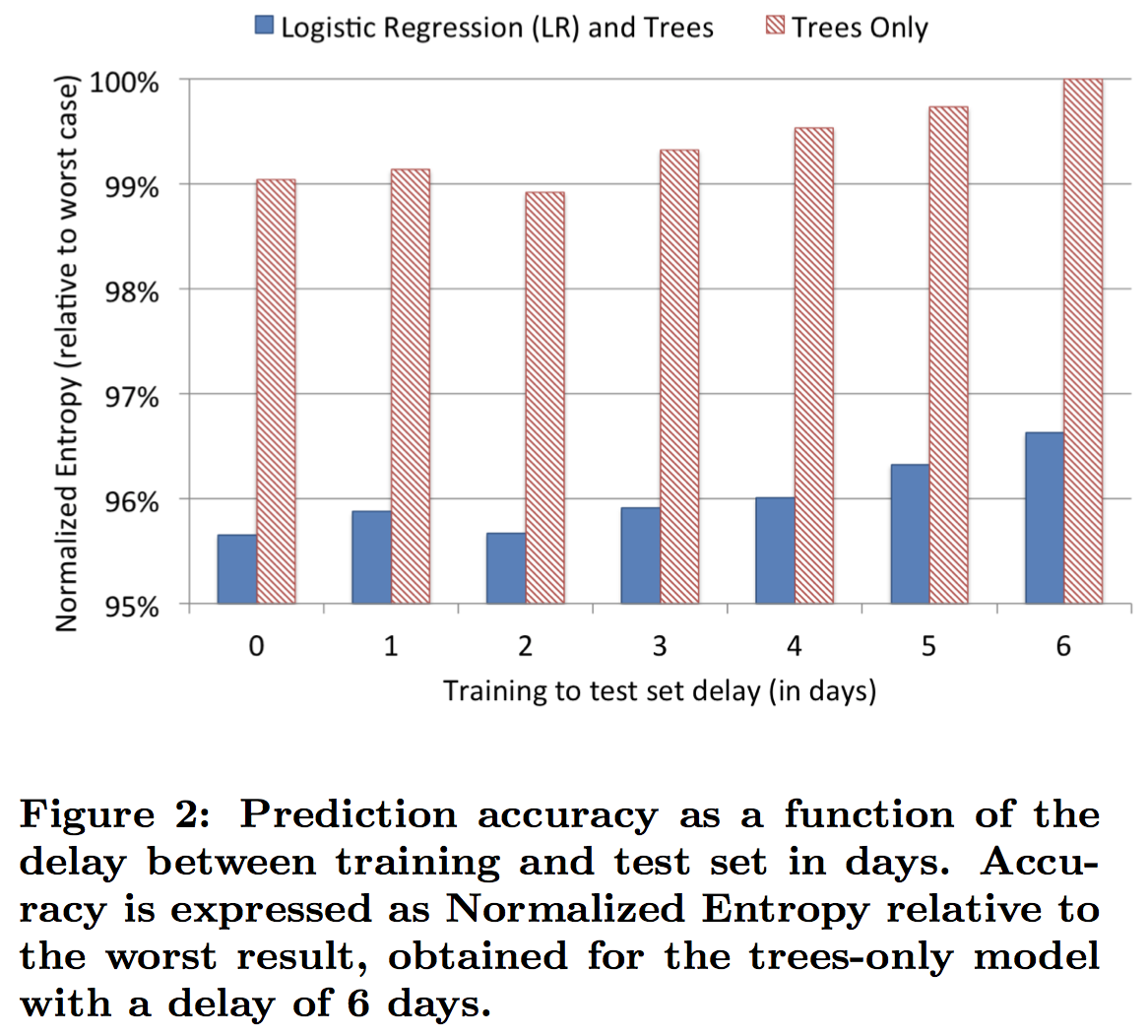
图3 Normalized Entropy vs delay
因此,为了提升模型的指标,需要提高data freshness,即进行online learning,其工作流程如图4所示。
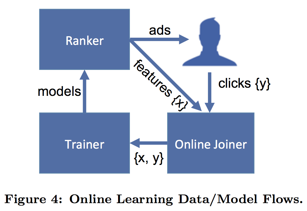
图4 online learning
一个online learning模块主要涉及到实时特征提取和模型实时训练这两个部分,其中实时特征提取部分对应于该论文中的online data joiner,而在decision trees + logistic regression模型结构中,模型实时训练部分主要针对logistic regression的近实时训练(decision trees仅用于feature transformation,不需要实时训练)。
3. 其他因素
-
Number of boosting trees
影响feature transformation后新特征的维度
-
Boosting feature importance
用于评估特征的重要性,可用于特征筛选
-
Historical features vs Contextual features
测试结果表明,Historical features(历史操作行为特征)比Contextual features(上下文信息,如用户所使用的终端等)作用更大;而Contextual features可用于处理cold-start问题
-
Sampling
- Uniform subsampling
- Negative down sampling
4. 总结
模型层面:
- Data freshness matters
- Transforming real-valued input features with boosted decision trees significantly increases the prediction accuracy of probabilistic linear classifiers
- LR with per-coordinate learning rate, which ends up being comparable in performance with BOPR, and performs better than all other LR SGD schemes under study
细节层面:
- The tradeoff between the number of boosted decision trees and accuracy
- Boosted decision trees give a convenient way of doing feature selection by means of feature importance
- For ads and users with history, historical features provide superior predictive performance than context features
总体来说,该论文给出的decision trees + logistic regression模型结构不但显著提升了CTR指标,而且在一定程度上减少了特征工程的工作量,该模型的几个优化点如下:
- 在特征维数特别大或数据集特别大的情况下,使用
decision trees进行feature transformation性价比不高,即训练较耗时且效果不一定很好 - 仍需要对Historical features做一定的特征工程
# 实现范例
# 来源:http://scikit-learn.org/stable/auto_examples/ensemble/plot_feature_transformation.html
import numpy as np
np.random.seed(10)

import matplotlib.pyplot as plt

from sklearn.datasets import make_classification
from sklearn.linear_model import LogisticRegression
from sklearn.ensemble import GradientBoostingClassifier
from sklearn.preprocessing import OneHotEncoder
from sklearn.model_selection import train_test_split
from sklearn.metrics import roc_curve
from sklearn.pipeline import make_pipeline

n_estimator = 10
X, y = make_classification(n_samples=80000)
# 划分数据集
X_train, X_test, y_train, y_test = train_test_split(X, y, test_size=0.5)
X_train, X_train_lr, y_train, y_train_lr = train_test_split(X_train,
                                                            y_train,
                                                            test_size=0.5)

grd = GradientBoostingClassifier(n_estimators=n_estimator)
grd_enc = OneHotEncoder()
grd_lm = LogisticRegression()

grd.fit(X_train, y_train) # GBDT
grd_enc.fit(grd.apply(X_train)[:, :, 0]) # GBDT feature transform
grd_lm.fit(grd_enc.transform(grd.apply(X_train_lr)[:, :, 0]), y_train_lr) # LR

y_pred_grd_lm = grd_lm.predict_proba(grd_enc.transform(grd.apply(X_test)[:, :, 0]))[:, 1] # GBDT+LR做预测
fpr_grd_lm, tpr_grd_lm, _ = roc_curve(y_test, y_pred_grd_lm)

y_pred_grd = grd.predict_proba(X_test)[:, 1] # 只使用GBDT做预测
fpr_grd, tpr_grd, _ = roc_curve(y_test, y_pred_grd)

plt.figure(1)
plt.plot([0, 1], [0, 1], 'k--')
plt.plot(fpr_grd, tpr_grd, label='GBT')
plt.plot(fpr_grd_lm, tpr_grd_lm, label='GBT + LR')
plt.xlabel('False positive rate')
plt.ylabel('True positive rate')
plt.title('ROC curve')
plt.legend(loc='best')
plt.show()

plt.figure(2)
plt.xlim(0, 0.2)
plt.ylim(0.8, 1)
plt.plot([0, 1], [0, 1], 'k--')
plt.plot(fpr_grd, tpr_grd, label='GBT')
plt.plot(fpr_grd_lm, tpr_grd_lm, label='GBT + LR')
plt.xlabel('False positive rate')
plt.ylabel('True positive rate')
plt.title('ROC curve (zoomed in at top left)')
plt.legend(loc='best')
plt.show()